LayOpt: User Guide
Introduction
LayOpt is an interactive web application that allows users to rapidly identify the optimal layout of a truss (pin jointed frame). The goal is to find the minimum volume truss that can transmit a set of loads back to a set of supports. The truss is constrained to lie within a specified region, the design domain. The design domain can be of any polygonal shape and can include holes where structure is not permitted to lie.
Problems can involve single or multiple load cases. When multiple load cases are involved LayOpt seeks to find the minimum volume truss using plastic design principles.
Guidance on using the software is provided in the Usage section below. More information on the theory and methods underpinning LayOpt are described in the Theory and Methods section.
Usage
The Main Menu
The main menu provides access to core LayOpt operations, allowing you to set up a new problem, or to save or load an existing problem - a number of prebuilt example problems are available. A problem can be saved as an xml file that can be reopened and solved or edited later. Alternatively a shareable link for a given problem can be generated and shared with others.
Solutions can also be saved as images, with the type of image selectable via options in the menu. A filename can also be specified. Clicking "Save now" will generate and download the image according to the current specification.
The Tool Bar
The toolbar contains the tools that allow you to draw a structural problem on the canvas and to obtain the optimal (minimum volume) truss layout. Click a tool for more details on its use.
Edit
Grid
Domain
Loads
Supports
Solve
Simplify
Theory and Methods
Background
LayOpt makes use of mathematical optimization methods to obtain a minimum volume truss structure for a given problem. This section provides a brief introduction of the theory of absolute minimum material design and more information about the methods used in the web app.
Theory
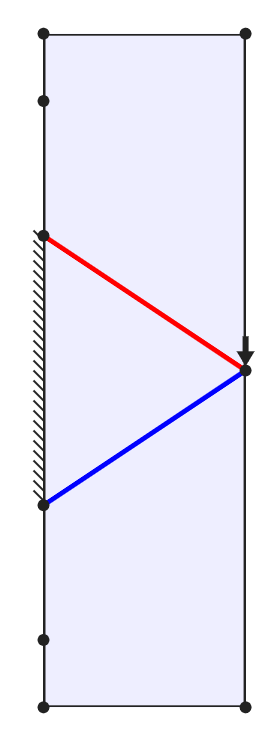
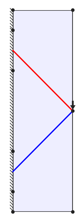
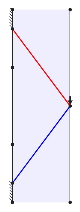
The theory behind absolute minimum volume structures has recieved academic interest for over a century. A seminal paper in the field was published by Michell (1904), leading to the emergence of so-called Michell structures. The rules governing such structures are seemingly simple, yet the resulting structures can be very complex. For example, members in tension and compression should always intersect at right angles, so that they are not working against each other. A very simple example is shown below; the central solution allows the minimum volume of material to be used. When the members form an angle less than 90 degrees, the force in each member is increased, leading to a higher volume. Conversely, when the angle is greater than 90 degrees, the force in the members is reduced but their length is increased.
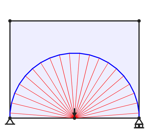
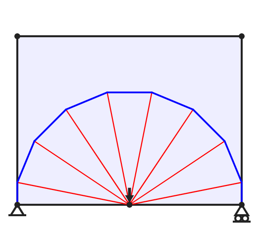
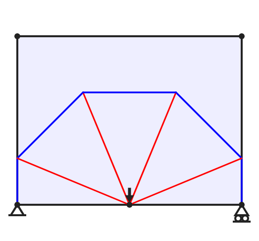
For most problems, ensuring that all members meet at right angles requires families of curved members. Generally there will be infinitely many, infinitessimaly thin such members. For example, a vertical load applied midway between two supports will be supported by a half wheel form, with a semi-circular outer member and infinitely many 'spokes' connecting to the central loaded point. Clearly, a structure with infinitely many members will not be practical to construct; however, structures of a similar layout but consisting of fewer members may have structural volumes only a few percent above the true optimum solution. The figure below shows approximations to the bicycle wheel type structure; the true minimum volume solution for this problem with unit limiting stress in tension and compression is pL / 2, where in this case the span L is 16, leading to a solution of 25.133.
Methods
Layout Optimization
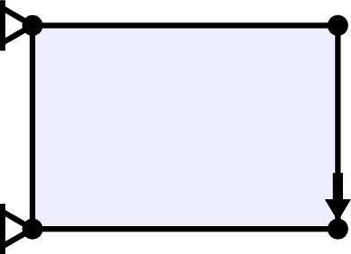
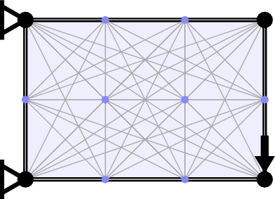
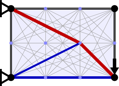
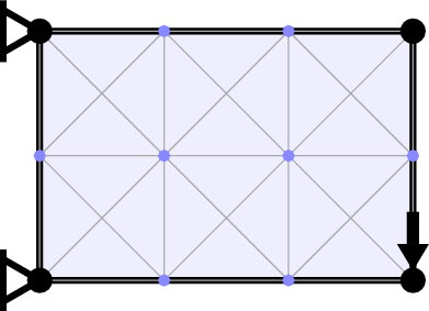
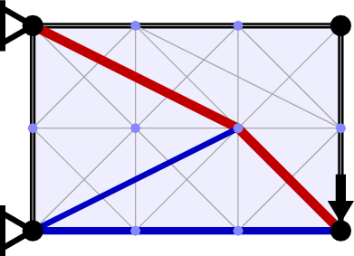
It was realized in the 1960s that minimum volume structures could be identified computationally. The steps in the numerical layout optimization procedure used by LayOpt are shown in the image below. First, the design domain (the region within which the structure is permitted to lie) is populated with nodes. Each pair of nodes is then connected with a potential structural member to create a "fully connected ground structure". Finally, a mathematical optimization problem is solved to identify the minium volume subset of members and their sizes.

The associated mathematical optimization problem turns out to be a very simple "linear programming" problem, as first outlined by mathematicians Dorn, Gomory and Greenberg (1964). The objective function is to minimize the total volume of material, which is calculated by summing the cross sectional areas of each member multiplied by its length. To ensure that the structure is able to carry the specified loads back to the supports, various constraints are required. Firstly, the forces at each node must be in equilibrium, i.e. the total force at each node must sum to zero in both the horizontal and vertical directions. Secondly, each member must have a cross sectional area that is large enough to carry the force being transmitted. This is calculated based on the given permitted limiting material stress in tension and compression.
In LayOpt, nodes are located at the intersections of grid lines, and at locations where the grid lines cross the edges of the design domain. The coarseness of the grid can be adjusted using the slider. When a very fine nodal grid is employed a very close approximation of the true minimum volume is obtained. However, increasing the number of nodes also increases the computational resources required, and usually the complexity of the resulting structure.
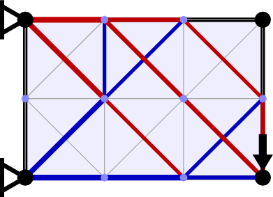
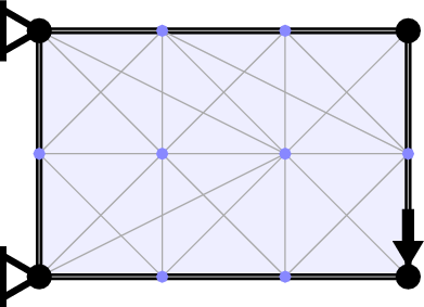
To increase the computational efficiency LayOpt makes use of the adaptive member adding method proposed by Gilbert and Tyas (2003). This only requires a subset of the possible connections to be considered initially (here only adjacent nodes are initially connected). Once this problem is solved, each initially neglected potential member is checked to see if it is likely to reduce the calculated volume. If so, then is considered for addition to the problem in the next iteration. This process continues until no potential members can be found that have the potential to reduce the volume of the structure. At this point the volume of the structure will be identical to the solution of the corresponding problem which included all potential member connections from the outset. LayOpt shows the result of each member adding iteration as it is calculated, allowing you to see how the optimal design is being identified.
Geometry Optimization
In the layout optimization stage, joint locations are prededined, lying only at the predefined locations described in the previous section. A geometry optimization rationalization step that involves moving the positions of joints can be used to improve the solution obtained via layout optimization, i.e. joints are added as variables in the optimization.
The mathematical formulation of the geometry optimization phase is similar to the layout optimization phase, although the resulting optimization problem is now non-linear. The objective is still to minimize the volume, and there are still constraints on equilibrium and allowable stresses; additionally, each joint is given a maximum distance that it may move in each iteration. LayOpt displays the results of each iteration as they are calculated, and it is possible to see nodes gradually moving to their new positions in LayOpt. Joints that move too close together are merged, and new joints are added at locations where members cross over one another.
Simplification
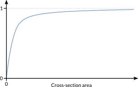
The simplification method employed by LayOpt is based on a simple function which represents the existence of each member (He et al., 2018). The function is based on the cross-sectional area of a member, and has a value of 0 when the member has a zero cross-sectional area, and a value close to 1 when the cross-sectional area of the member is large. Therefore, by summing this function over all potential members in the structure, we obtain an approximation of the number of members that exist.
This function can then be used as an objective for the optimizer, i.e. the problem becomes to minimise the approximate number of members (whilst maintaining the equilibrium and stress constraints from the previous stages). To prevent the solver obtaining solutions that are overly simple and overly heavy, a constraint on the maximum permitted increase in volume is added. This can be set using the slider in LayOpt.
Finally, to ensure that the lightest version of the simplified solution is obtained, geometry optimization is performed on the resulting simplified structure.
Modelling Assumptions
This section briefly considers other modelling assumptions made in LayOpt.
Truss structures
All members carry only axial forces, i.e. tension or compression but not bending. Beams in bending can be effectively modelled as two axial members (along the top and bottom chords), linked by suitable truss members. This has the advantage of providing the optimal structural depth, with the optimal distribution of material also identified.
Material idealization
LayOpt uses a plastic material model. Many common engineering materials display plastic behaviour, including the majority of metals. Plastic behaviour means that when the material reaches a certain stress value, it will begin to deform and will maintain that value of stress.
For single load case problems, the layout of the minimum volume structure is the same for elastic or plastic material assumptions. In single load case problems, all members have an identical stress and strain (virtual strain in the plastic case) state, and changing from the plastic to the elastic solution simply requires scaling each member’s thickness by an appropriate factor. The optimal layouts for the elastic vs plastic material models only diverge when multiple load cases are considered.
References
Dorn WS, Gomory RE, Greenberg HJ (1964), Automatic Design of Optimal Structures, Journal de Mecanique, 3(1):24-52.
Gilbert M, Tyas A (2003), Layout optimization of large-scale pin-jointed frames. Engineering Computations, 20(8):1044-1064.
He L,.Gilbert M (2015), Rationalization of trusses generated via layout optimization, Structural and Multidisciplinary Optimization, 52(4):677-694.
He L, Gilbert M, Shepherd P, Ye J, Koronaki A, Fairclough HE, Davison B, Tyas A, Gondzio J, Weldeyesus AG (2018), A new conceptual design optimization tool for frame structures, In Proceedings of IASS Annual Symposia, International Association for Shell and Spatial Structures (IASS), 2018(19):1-8.
Michell AGM (1904), The limits of economy of material in frame-structures, Philosophical Magazine, 8(47):589-597.